Did you get lucky or unlucky?
Some bugs are flaky, appearing only at specific times, or when the system is in a particular state, or in the presence of problems like network faults, or some annoying combination of all of the above. These problems are particularly frustrating to debug because they’re so hard to hit in the first place. They frequently make it through testing undetected, only to appear in production where debugging becomes far more expensive and disruptive.
Antithesis finds these tricky bugs by running your software many times, while injecting different combinations of faults, to try and flush them out. Once we’ve found one, our deterministic simulation environment can perfectly reproduce it, allowing you to replay it as many times as you want. However, the process of finding rare bugs in the first place takes time. For any given level of testing effort, some bugs will lurk at the edge of discoverability, appearing in some of your test runs but not others.
It’s difficult to figure out when these rare bugs are fixed. Say that you put in what you hope is a fix and then do another test run. For most bugs, seeing your Antithesis test switch from red to green in the new run is a good indication that your fix worked. For a rare bug, this isn’t enough. Did you really fix the problem, or were you just “lucky” enough to avoid it this time?1
To help you figure this out, Antithesis provides extra information for rare bugs in your triage report. You’ll see extra findability information, with a graph that estimates how many more runs you’ll need to do before you can be confident that the problem has been fixed. Here’s an example:
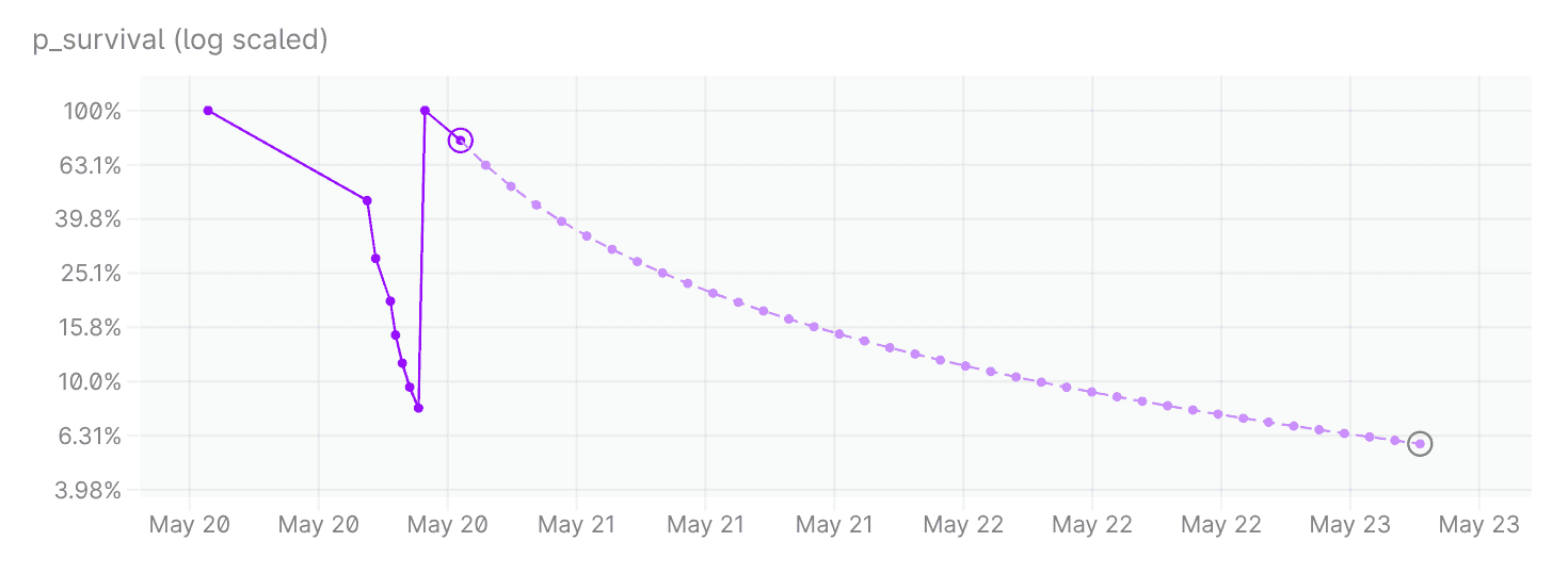
Each data point marks a test run. When we first encountered the bug (the leftmost point), the probability of the bug being present was 100%. It declined following a string of runs when we didn’t see the bug, only to jump back to 100% when we encountered it again. The most recent data point is circled in purple. Future runs are projected in lighter purple, assuming evenly spaced runs of the same length.
The y-axis shows what we’re calling p_survival, the probability that we could have tested for that long without seeing the bug, under the hypothesis that the bug still exists. If the bug does still exist, the probability of seeing it increases as we carry out more runs. Equivalently, the probability of not seeing the bug decreases. If we haven’t seen the bug, we say that we have “survived” so far.
The point with a green circle indicates the point where we reach 94% confidence that the bug is no longer there.
To understand how we create this graph, we’ll start simpler. As a first measure of findability, we’ll estimate a mean time-to-bug: the mean CPU time it takes to find a bug in a given test run. First, though, let’s make a quick detour to discuss what “time” can mean in Antithesis, as this can be a confusing topic.
Time vs. time vs. time
There are three types of time relevant to Antithesis: CPU time, wall-clock time, and vtime. The first two are in common use, whereas vtime is Antithesis-specific.
We’ve already mentioned CPU time. CPU time is the time that a central processing unit spends actively working, as opposed to sleeping or idling.
Wall-clock time is the actual time taken from the start of a task to the end. CPU time may be less than wall-clock time, for instance because the task needs to wait for other processes to finish. On the other hand, if the task is running in parallel on multiple CPUs, CPU time can be many times longer than wall-clock time. In Antithesis, we fuzz using every core of the machine, each of which is simulating its own parallel timeline.
Antithesis also has a concept of simulated time within each timeline. We call this vtime (short for “virtual time”), and in general it also runs differently to wall-clock time. This is the time that your program measures — for example, if it sleeps for one second, then one second of vtime will elapse. Our multiverse map is essentially a tree of all the timelines with the horizontal axis given in vtime:
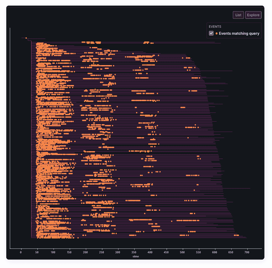
In this post, we’re mostly going to be concerned with CPU time, as this is what we use to get a measure of how much testing Antithesis needs to do to find a bug. However we’ll also need to take into account the branching structure of the multiverse, as we’ll see in the next section, so it’s useful to know about vtime too.
Estimating mean time-to-bug
The simplest possible thing we could do to estimate mean time-to-bug is to ignore the whole concept of branches and divide the total CPU time by the total number of bugs seen across all timelines.
Unfortunately, this won’t give us a very good estimate. To see why, let’s look at a simplified version of the multiverse map. A real multiverse map has a lot more branches, but here we’ll just draw a few:
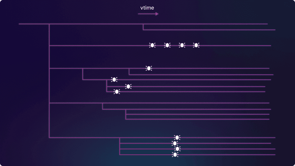
You can see that there’s a single branch at first, and then there’s a “root moment” in vtime where the tree first splits into branches (five of them, in this simplified case). This is where the fault injector first gets turned on — from this point on, the branches will differ as different faults occur in different timelines. Each of these branches from the root moment is the start of a subtree which may branch further.
Once we’re inside a subtree, we can’t expect bugs in different branches of the subtree to be independent of each other. There might be some fault that “bakes in” the bug for all branches of the subtree (you can see this happen in the bottom subtree in the picture above). So we can only really count the first instance of the bug that we see in each subtree:2
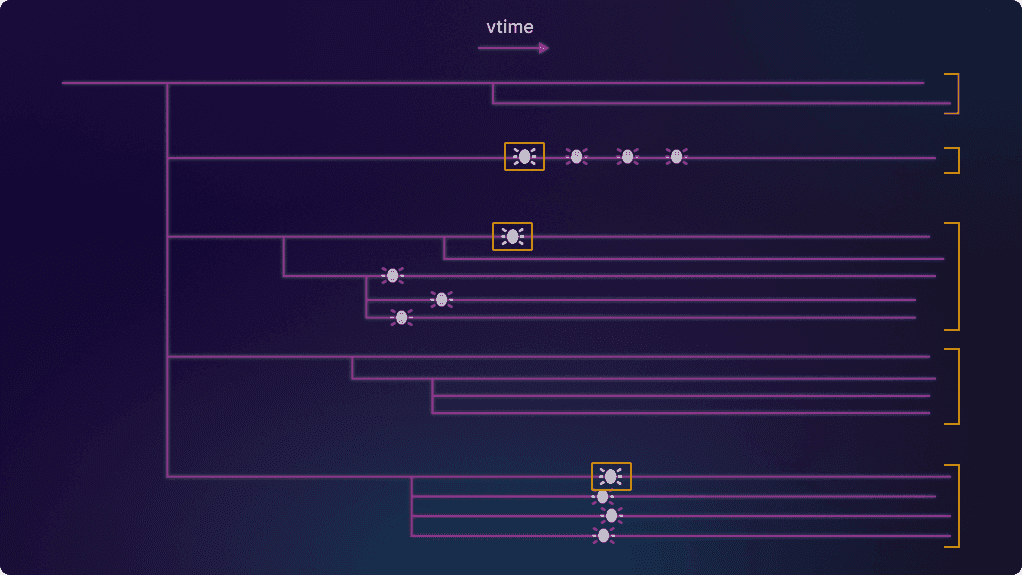
We’ll take the CPU time spent in each subtree up to the moment of the first bug (this will cover multiple branches if the bug isn’t found in the first branch). If there’s no bug, we’ll take the whole subtree. In our example above, this gives us five time intervals, three where we saw the bug and two where we didn’t. The following diagram shows the time intervals as solid bars, with dotted lines showing the rest of the time spent in each subtree.
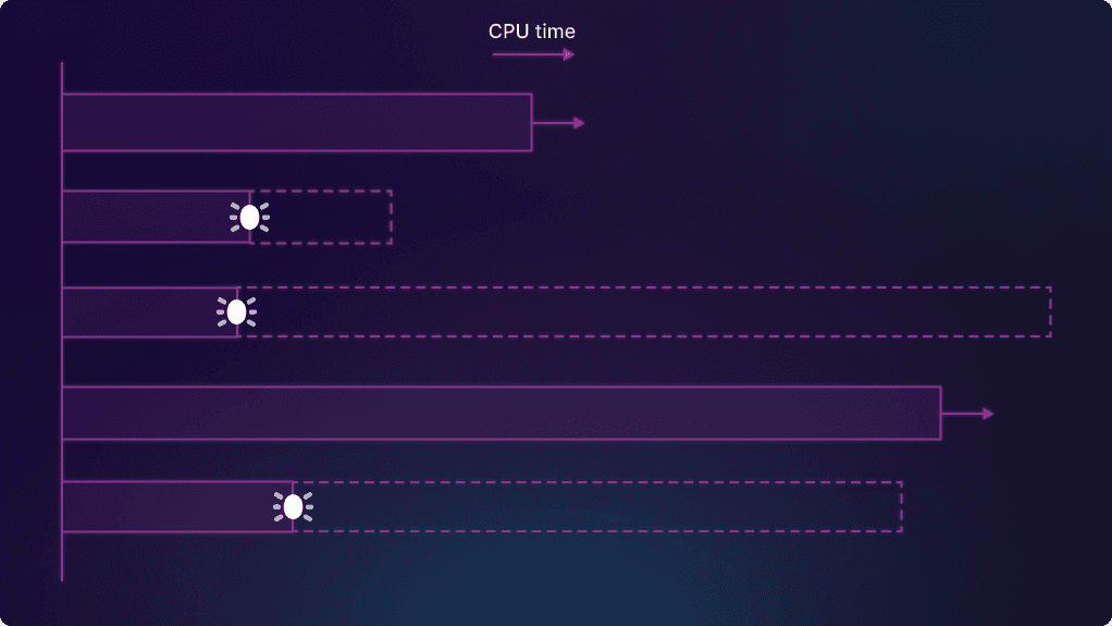
If we’d seen the bug in all the branches, we could get a mean time-to-bug by just adding up all the time intervals to get a total time
The classic example question in survival analysis is “how long will the average patient in this study survive?”, with incomplete information because (hopefully!) some patients survive past the end of the study. We instead have the question “how long until we see the bug?”, and we have incomplete information because some subtrees end before we find it. (The survival analysis framework assumes that you’d eventually see the bug.)
How we should account for the incomplete runs depends on what we expect the distribution of the CPU time to first bug in a subtree to look like. We’ll assume that first bugs occur independently, so that the time to first bug in one subtree doesn’t affect the time to first bug in another subtree, and at a constant average rate
For example, if you saw 1 bug in a 200 CPU hour run, your total survival time
For an exponential distribution, we can make a surprisingly simple estimate of the mean time-to-bug. Say you have
Notice that for common bugs that you find in every subtree,
Back to the findability graph
Now we’re ready to go back to the original question of how long we have to wait to be confident we’ve fixed the bug.
Let’s look at the findability graph from the beginning of the post again:

To create this graph we want to calculate a probability p_survival for each run that the bug is still there, and when this drops low enough we’ll count it as fixed.
For a run in which we saw the bug, calculating p_survival is easy. We have p_survival = 1 because no time has yet passed since we saw the bug.
Now let’s take a run where you didn’t see the bug. This is where the calculation from the previous section comes in. We found the most likely value of the rate parameter
As a first rough estimate, we can plug in this value of p_survival.
However, we actually do something a bit more complicated. The value of
Once we do that, we find that the curve is a mixture of exponential distributions that has a heavier tail than a single exponential distribution, meaning that it decays more slowly.4 This gives us more conservative estimates for when the bug is fixed than exponential decay, which is useful because rare bugs that reoccur in production are scary and we want to be sure that they’re definitely fixed.
Taking the example we used before of a total survival time
There’s one extra complication. Each point on the graph represents a different run, and you might have made changes to your system between runs, altering the frequencies of bugs that you see. To help account for this, we take a weighted average of data from multiple runs to calculate total values for
We now have all the pieces we need to understand the findability graph. We’ve already discussed the projected decay curve. You can also see similar decay behaviour for the existing runs. The difference is that these are real runs rather than projected ones, so they are spaced out variably in time and the shape of the curve is less obvious. They also have a different decay rate as the calculated value of
Deciding when to stop looking
In software testing, we’re always in the difficult position of trying to prove a negative. We can prove that a bug still exists by finding it, but if we don’t find it we still can’t say with absolute certainty that it’s gone. This is frustrating when you just want to know that your software really, truly, for sure has no bugs. But certainty is a high bar, and very little meets that standard of proof.
From a practical point of view, what we can do is quantify how much testing we need to do to have confidence that your flaky bug is gone, and then throw that amount of disruption at your system. In the course of each overnight Antithesis test run, your system experiences the equivalent of years or decades of production chaos. The findability graph is a guide to how much chaos is enough.
If you’ve found yourself interested in findability, you might also like to find out more about how Antithesis works. See our video Antithesis in less than 5 minutes.


